Exit Cap Rates vs. Growth Rates in Terminal Value
In commercial real estate, terminal value is a critical part of property valuation, often making up 60–80% of the total value in a discounted cash flow (DCF) model. It’s calculated using two methods:
Exit Cap Rate Method: Applies a capitalization rate to the projected net operating income (NOI) at the time of sale.
Formula: Terminal Value = NOI ÷ Exit Cap Rate
Example: $500,000 NOI ÷ 6.5% cap rate = $7,692,308.
Perpetuity Growth Method: Assumes cash flows grow indefinitely at a steady rate.
Formula: Terminal Value = (Final Year Cash Flow × (1 + Growth Rate)) ÷ (Discount Rate – Growth Rate)
Example: $400,000 cash flow × 1.03 ÷ (8% – 3%) = $8,240,000.
Quick Comparison
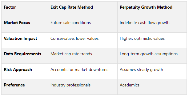
Both methods are sensitive to assumptions. Small changes in cap rates or growth rates can significantly impact terminal value. For balanced results, investors often use both methods and average the outcomes. Sensitivity analysis is essential to test how different assumptions affect valuations and to ensure realistic projections.
Exit Cap Rates Explained
Definition and Formula
An exit cap rate, often called a terminal cap rate or reversion cap rate, is the expected rate of return used to estimate what a property might sell for at the end of your investment period. It links the projected net operating income (NOI) to the estimated sale price.
Here’s the formula for calculating the terminal value:
Terminal Value = Projected Net Operating Income (NOI) ÷ Exit Cap Rate
For instance, if you expect a property to generate $500,000 in NOI in the year you plan to sell and apply a 6.5% exit cap rate, the terminal value would be $7,692,308 ($500,000 ÷ 0.065).
Exit cap rates focus on future market conditions at the time of sale. Typically, they are set higher than entry cap rates. A common guideline is to add 10 basis points (0.1%) for each year of the hold period.
The calculation depends on several factors, including market trends, property specifics, and location, which are discussed below.
Factors That Affect Exit Cap Rates
Several elements influence exit cap rates, and understanding them is essential for making accurate projections.
Market and Economic Conditions are the primary drivers of exit cap rates. Interest rates, inflation, and economic cycles all play significant roles. For example, when interest rates rise, cap rates usually increase as investors seek higher returns to offset higher borrowing costs. Market sentiment also matters - strong markets often experience cap rate compression, while weaker or recessionary markets see cap rate expansion.
Property characteristics also shape exit cap rate assumptions. Newer properties tend to have lower cap rates due to reduced maintenance costs and modern features. The property type is another consideration: apartment buildings often maintain stable cap rates because of consistent housing demand, while industrial properties benefit from e-commerce growth. On the other hand, office spaces are influenced by changing workplace trends, and those that meet modern environmental standards may achieve lower cap rates.
Location is another key factor. Properties in high-demand urban areas usually have lower cap rates due to economic stability and strong demand, whereas properties in smaller, riskier markets may require higher cap rates to reflect greater uncertainty. Local factors like population growth, job opportunities, infrastructure projects, regulatory policies, and the supply pipeline in the submarket should all be analyzed.
In commercial real estate, exit cap rates generally fall between 3% and 10%. To set a realistic exit cap rate, start with current market cap rates for comparable properties. Then, adjust based on expected market changes, the property’s future condition, anticipated competition, and projected supply and demand.
Growth Rates in Terminal Value Calculations
Definition and Formula
The perpetuity growth rate reflects the constant rate at which a property's free cash flows are expected to grow indefinitely. Unlike exit cap rates, which focus on market conditions at the time of sale, this approach assumes the property will continue generating increasing cash flows beyond the forecasted period.
Here’s the formula for calculating terminal value using the growth in perpetuity method:
Terminal Value = (Final Year Cash Flow × (1 + Growth Rate)) ÷ (Discount Rate – Growth Rate)
For instance, if a property generates $400,000 in cash flow during its final forecasted year, with a perpetual growth rate of 3% and a discount rate of 8%, the terminal value would be:
($400,000 × 1.03) ÷ (0.08 - 0.03) = $8,240,000
This method differs from the exit cap rate approach, which estimates the property's sale price at a specific future point.
When determining an appropriate growth rate, metrics like GDP growth or the risk-free rate are often used as benchmarks. Generally, long-term growth rate assumptions fall between 2% and 4%, reflecting sustainable economic trends. Even small changes in these rates can significantly affect terminal value, making precision essential.
Why Accurate Growth Rate Forecasting Matters
Growth rate assumptions are a cornerstone of terminal value calculations, as terminal value often accounts for about 75% of the total valuation in a discounted cash flow (DCF) model. Because of this, even slight adjustments to growth rates can lead to substantial shifts in a property's valuation. To avoid inflated projections, conservative estimates are vital.
Typically, the terminal growth rate aligns with historical inflation (2%-3%) or GDP growth rates (3%-4%). A higher growth rate - exceeding average GDP growth - implies the property will outperform the overall economy indefinitely, a claim that requires strong justification. For context, growth rates above 5% are generally seen as unsustainable.
The interaction between a property's return on capital and its cost of capital also plays a role. If the return on capital surpasses the cost of capital during the stable growth period, increasing the growth rate tends to boost value. However, if these rates are equal, raising the growth rate has little to no impact.
Given the uncertainty of long-term forecasts, sensitivity analysis becomes crucial. Testing different growth rate scenarios helps evaluate their effects on potential returns and risk exposure. This approach underscores the importance of selecting the right method - whether perpetuity growth or exit cap rate - for DCF models in commercial real estate.
DCF Analysis Part 4: Final Valuation - and Sensitivity Analysis!
Transform Your Real Estate Strategy
Access expert financial analysis, custom models, and tailored insights to drive your commercial real estate success. Simplify decision-making with our flexible, scalable solutions.
Exit Cap Rates vs. Growth Rates: Direct Comparison
Building on earlier discussions of terminal value methods, let’s dive into a direct comparison of exit cap rates and growth rates.
How the Calculation Methods Compare
The key difference between these two methods lies in their assumptions and calculations. The exit cap rate method focuses on the property’s potential sale value at a specific future date, while the perpetuity growth method assumes the property generates cash flows indefinitely.
Here’s how they work:
Exit Cap Rate Method: This calculates terminal value using the property’s final year's Net Operating Income (NOI) and a market-derived cap rate. For example, with a projected NOI of $500,000 in year 10 and an 8% exit cap rate, the terminal value would be $6,250,000.
Perpetuity Growth Method: This applies a constant growth rate to the final year’s cash flow, dividing it by the difference between the discount rate and growth rate. Using the same $500,000 cash flow, a 3% growth rate, and an 8% discount rate, the terminal value would be $10,300,000.
The exit cap rate method provides a more straightforward, linear reaction to changes. In contrast, the perpetuity growth model is highly sensitive to small adjustments in the discount and growth rates. Industry professionals often lean toward the exit multiple approach, while academics typically favor the perpetual growth model for terminal value calculations.
Key Differences and When to Use Each Method
Choosing the right method depends on market conditions and your investment strategy. Here’s a breakdown:
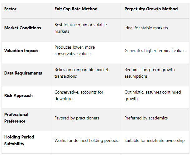
For uncertain markets, the exit cap rate method offers a buffer against unforeseen risks. In more stable environments, focusing on NOI growth while incorporating conservative cap rate assumptions provides a well-rounded view of potential value. On the other hand, when fundamentals are strong and rental growth looks sustainable, the perpetuity growth method can capture additional value that the exit cap approach might miss.
Since terminal value often accounts for 70% to 80% of the total net present value in discounted cash flow analyses, the choice of method can significantly impact investment decisions. Generally, the perpetuity growth model yields higher values than the exit multiple method, which is why conservative investors often prefer the latter.
To strike a balance, many experienced investors calculate terminal value using both methods and average the results. This dual approach acknowledges that neither method is perfect but helps provide a realistic range of outcomes. For instance, The Fractional Analyst incorporates both methods into its underwriting models, enabling robust scenario testing and deeper insight into valuation drivers. This combined strategy is especially useful for sensitivity analyses, offering a clearer picture of how different assumptions could influence investment outcomes.
Sensitivity Analysis of Terminal Value Assumptions
Since terminal value often makes up more than half of a DCF's total value, it’s crucial to understand how sensitive these calculations are to your key assumptions. This step connects the theoretical methods for calculating terminal value to their practical applications in financial modeling.
Why Sensitivity Analysis Matters
Terminal value calculations are incredibly sensitive to even minor changes in variables. For instance, a 50 basis point shift in the discount rate or exit cap rate can lead to a 12.1% change in value. A real-world example is Blackstone REIT, where the NAV per Class I share rose from $10.4493 in April 2020 to $14.9680 by April 2022 - a 43% increase. About one-fourth of this growth was attributed to lower discount and cap rates.
This level of sensitivity highlights the vulnerability of DCF models to assumption changes. Sensitivity analysis helps investors gauge the range of possible outcomes and strengthens confidence in their decisions.
Best Practices for Sensitivity Testing
To conduct effective sensitivity analysis, consider these practical tips:
Base assumptions on reliable market data. Use current market trends and historical data to guide your inputs. For terminal growth rates, a range of 2.0% to 4.0%, with an average around 3.0%, is typically aligned with GDP growth expectations.
Prioritize high-impact variables. Focus on key factors like exit cap rates and growth rates. When adjusting these, limit changes to 0.5% or less to keep assumptions realistic.
Leverage Excel for quick analysis. Excel’s data table feature allows you to efficiently model how individual or combined variable changes affect terminal value.
Incorporate stress testing. Test your assumptions under various scenarios - ranging from worst-case to optimistic - to see how the model performs in different economic conditions.
Identify unrealistic outcomes. If terminal value seems disproportionately large, consider extending the forecast period or revising other assumptions.
Blend data with market expertise. While sensitivity analysis provides valuable insights, refine your assumptions by consulting industry experts and incorporating current market knowledge.
Present results clearly. Ensure your findings are easy to interpret, especially when significant variations arise from changes in assumptions.
Key Takeaways
Main Points Summary
When calculating terminal value, it's crucial to differentiate between exit cap rates and perpetual growth rates. Exit cap rates estimate the projected sale price by dividing forecasted Net Operating Income (NOI) by an anticipated future cap rate. On the other hand, growth rates assume that terminal cash flows will grow indefinitely at a steady rate. Both approaches play a major role in determining valuation outcomes.
In practice, exit multiples are often preferred by industry professionals, while academics tend to favor the perpetual growth model. A balanced approach uses both methods for cross-checking results. When estimating exit cap rates, many investors apply a premium of 1% to 2% over the initial cap rate, while keeping assumptions conservative.
Even small adjustments in cap rates can lead to significant changes in Internal Rate of Return (IRR). This highlights the importance of precision in financial modeling - a skillset that The Fractional Analyst specializes in.
How The Fractional Analyst Supports CRE Professionals

The Fractional Analyst is designed to simplify the complexities of terminal value calculations for commercial real estate (CRE) professionals. By addressing the nuances of sensitivity analysis and method comparisons, we help ground exit cap and growth rate assumptions in reliable market data.
Our CoreCast platform offers cutting-edge real estate intelligence tools that streamline terminal value assessments, empowering better decision-making. In addition, we provide free financial models, such as multifamily acquisition templates and IRR matrices, complete with built-in sensitivity analysis for testing various scenarios.
Whether you need expert analyst support for one-off projects or ongoing market research and investor reporting, The Fractional Analyst delivers the precision and insights required to refine terminal value calculations and enhance investment returns in today’s ever-changing CRE landscape.
FAQs
-
Exit cap rates and perpetuity growth rates play a crucial role in determining the terminal value within a discounted cash flow (DCF) model. Even small adjustments to the growth rate (g) can create noticeable shifts in valuation, especially when the growth rate gets close to the discount rate. This proximity can make the model more sensitive and prone to fluctuations.
The exit cap rate also has a direct impact on terminal value by defining the multiple applied to stabilized cash flows. A higher cap rate lowers the terminal value, while a lower cap rate increases it. These inputs are especially important during sensitivity analysis, as even minor tweaks can lead to significant changes in valuation results. Choosing these assumptions thoughtfully is key to building a model that delivers accurate and dependable outcomes.
-
When deciding between the exit cap rate method and the perpetuity growth method, the choice often hinges on the state of the market and the specifics of the investment. In markets that are stable or experiencing a decline, a higher exit cap rate is typically applied. This accounts for aging assets and greater risk, offering a more cautious projection of terminal value. On the other hand, in thriving or appreciating markets, a lower exit cap rate is often more fitting, reflecting stronger property values and greater investor confidence.
In times of market uncertainty or volatility, performing a sensitivity analysis becomes essential. This process lets you evaluate how shifts in exit cap rates or growth rates influence terminal value, equipping you with the insights needed to make smarter and more adaptable investment decisions.
-
Sensitivity analysis gives investors a way to test how changes in critical assumptions - like exit cap rates and growth rates - affect terminal value calculations. By tweaking these variables and reviewing the results, investors can pinpoint which factors carry the most weight in the valuation and identify potential areas of risk.
This method ensures that assumptions remain grounded in reality and reflect current market trends, offering a more accurate view of an investment's potential. It also enables smarter decision-making by showing how much the valuation might shift under different scenarios.