
How To Calculate Discount Rate in DCF
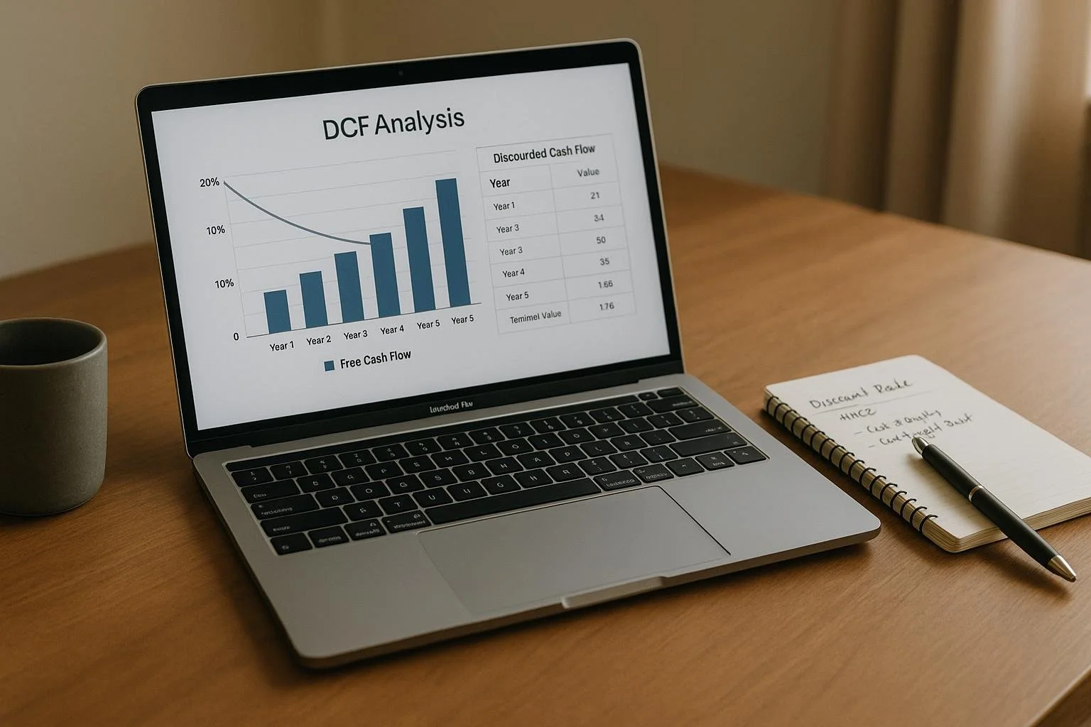
The discount rate in Discounted Cash Flow (DCF) analysis is a key metric used to convert future cash flows into their present value, accounting for risks and the time value of money. In commercial real estate, it helps investors evaluate whether a property aligns with their financial goals by reflecting the risks tied to location, tenant stability, lease terms, and market conditions.
Key Takeaways:
- Definition: The discount rate is the minimum return an investor expects, balancing risks and time.
- Formula: Present Value (PV) = Future Cash Flow (CF) ÷ (1 + Discount Rate)^Years.
- Importance: A higher discount rate reduces the present value, reflecting higher risk; a lower rate increases it.
- Factors to Consider:
- Projected cash flows (e.g., Net Operating Income with rent escalations and vacancy assumptions).
- Terminal value (future sale price) using an exit cap rate.
- Risk adjustments for property specifics, market conditions, and financing.
Methods to Calculate Discount Rate:
- Required Rate of Return: Start with a base rate and add premiums for risks like location or tenant concentration.
- Market-Based Approach: Use comparable sales and cap rates to infer the discount rate.
- Risk-Adjusted Approach: Add premiums to a risk-free rate (e.g., Treasury rate) for real estate, property, and market risks.
Example:
For a property generating $100,000 annually in five years, with a 9% discount rate, the present value is $64,993. Choosing the right discount rate ensures accurate valuations and smarter investment decisions.
Tools:
- Excel functions like NPV and IRR simplify calculations.
- Sensitivity tables help test how varying discount rates affect results.
- Software like The Fractional Analyst offers advanced modeling and real-time market data.
Accurate discount rate calculations are essential for reliable DCF analysis, ensuring your investment decisions reflect both current market conditions and property-specific risks.
How To Choose a Discount Rate in Real Estate Investment Analysis
Key Components for Calculating the Discount Rate
To calculate an accurate discount rate, you need to analyze key property and market inputs. These factors come together to create a detailed picture of the investment's risk profile and expected returns.
Projected Cash Flows and Holding Period
The starting point for discount rate calculations is reliable cash flow projections. For commercial real estate, this typically begins with the property’s Net Operating Income (NOI) - the rental income after deducting operating expenses like property management fees, maintenance costs, insurance, and property taxes.
Most commercial real estate investors plan for a holding period of 5 to 10 years. Office buildings and retail properties often lean toward the longer end of this range, while properties needing repositioning or opportunistic investments may have shorter timeframes. The length of the holding period directly impacts the discount rate, as longer horizons require higher rates to account for increased uncertainty.
When projecting NOI, it’s common to include 2–3% annual rent escalations. For instance, if a property generates $500,000 in NOI in year one, a 3% escalation would bring year two’s NOI to $515,000.
Vacancy assumptions are equally important. Even well-leased properties should factor in some level of vacancy during the holding period. A conservative estimate might assume 5–10% vacancy for stable office properties. For retail properties in transitioning markets, higher vacancy rates of 15–20% might be more realistic.
Terminal Value and Exit Cap Rate
Once cash flows are established, the next step is calculating the terminal value, which often accounts for 60–80% of the total DCF value. This represents the expected sale price at the end of the holding period.
To determine the terminal value, you need an exit cap rate. This is calculated by analyzing current market cap rates and adjusting for potential changes over the holding period. For example, if similar properties in the market are trading at a 6.5% cap rate, you might assume a 7.0% exit cap rate to reflect possible market softening or the property aging over time.
It’s common practice to set the discount rate 100–300 basis points higher than the exit cap rate to account for risks tied to ownership, management, and market timing. For instance, with a discount rate of 9%, an exit cap rate between 6.5% and 7.5% would be reasonable.
The formula for terminal value is straightforward: divide the projected NOI for the year following the sale by the exit cap rate. For example, if the projected NOI in year eight is $600,000 and the exit cap rate is 7%, the terminal value would be $8,571,429 ($600,000 ÷ 0.07).
Risk Factors and Adjustments
Accurate discount rates also require adjustments for specific risks. These adjustments refine your calculations and ensure they reflect the unique challenges of the property and investment strategy.
Property-specific risks include factors like tenant concentration, lease expirations, and the property’s physical condition. For example, a property where 60% of income comes from one tenant might require a 100–200 basis point premium over a property with a more diverse tenant base. Similarly, properties with leases nearing expiration need higher discount rates to account for re-leasing risks.
The market where the property is located also plays a role. Primary markets like Manhattan typically have lower discount rates (8–10%) due to greater liquidity, while secondary markets might demand rates of 10–14%, influenced by local economic conditions such as job growth, population trends, and new supply pipelines.
The type of asset adds another layer of complexity. For instance, core office properties with long-term credit tenants might have discount rates of 7–9%, while value-add retail properties could require rates of 12–15%. Industrial properties, especially well-located warehouses, have become increasingly popular, with discount rates often falling between 6–8%.
If you’re using debt financing, you’ll need to adjust the discount rate to account for leverage risks. For example, if 70% of the purchase is financed with a 5% interest rate loan, the equity discount rate should reflect the additional financial risk. Many investors add 200–400 basis points to their unleveraged return when debt is involved.
Ultimately, the goal is to craft a discount rate that captures all risks while staying competitive. For further refinements and model validation, tools like those offered by The Fractional Analyst can provide valuable support.
Step-by-Step Guide to Calculating the Discount Rate
Now that we’ve broken down the key concepts, let’s dive into the calculations. The discount rate is a crucial part of any DCF (Discounted Cash Flow) analysis, so understanding how it works is essential. Below, we’ll walk through the core formulas and methods step by step.
Core Formulas Explained
The present value formula is your starting point. It’s used to convert future cash flows into their value today:
PV = FV ÷ (1 + r)^n
Here’s what each term means:
- PV: Present Value
- FV: Future Value
- r: Discount rate (expressed as a decimal)
- n: Number of years
For example, let’s say a property is expected to generate $100,000 in net operating income (NOI) three years from now, and your discount rate is 9%. Using the formula, the present value would be $77,218 ($100,000 ÷ 1.09³).
To take it a step further, the Net Present Value (NPV) formula sums up all discounted cash flows and subtracts the initial investment:
NPV = Σ [CFt ÷ (1 + r)^t] - Initial Investment
A positive NPV means the investment should exceed your required returns. For commercial real estate, investors often aim for NPVs between $500,000 and $1,000,000 on deals valued between $5 million and $20 million.
Another key metric is the Internal Rate of Return (IRR) - the discount rate that makes NPV equal zero. It’s a benchmark to assess whether your chosen discount rate aligns with your investment goals.
Methods for Determining the Discount Rate
There are three common ways to calculate your discount rate, each tailored to different strategies and market conditions.
- Required Rate of Return Method
This method begins with your target return and adjusts for specific risks. For example, institutional investors might start with a base rate of 6-8% for core properties and then add premiums for additional risks. A typical calculation might look like this:- 7% base rate
- +2% for a secondary market location
- +1% for tenant concentration risk
Total Discount Rate = 10%
- Market-Based Approach
Here, you analyze recent comparable sales to extract implied discount rates. For instance, if similar properties are selling at 6.5% cap rates with 3% annual NOI growth, the implied discount rate would be about 9.5%. This approach works best in active markets with frequent transactions, like office or retail properties in major cities. - Risk-Adjusted Approach
This method starts with a risk-free rate - like the 10-year Treasury rate (around 4.5% as of late 2024) - and adds premiums for various risks:- Real estate risk: 2-3%
- Property-specific risks: 1-3%
- Market risks: 1-2%
This systematic approach ensures you account for all relevant risk factors.
Discount rates vary by property type and location. For example:
- 7-9% for core assets (e.g., Class A office buildings with stable tenants)
- 9-12% for value-add properties needing upgrades or re-leasing
- 12-15% for opportunistic investments involving significant development or repositioning risks
Geography also plays a role. In primary markets like Manhattan or San Francisco, discount rates are often 100-200 basis points lower than in secondary markets due to higher liquidity and lower perceived risk.
Using Excel or Financial Tools
Once you understand the formulas, Excel becomes a powerful tool to simplify your calculations. It offers built-in functions like NPV, IRR, and XNPV that make DCF modeling much easier.
- NPV Function: The syntax is
=NPV(discount_rate, cash_flows) + initial_investment. Keep in mind, Excel assumes the first cash flow occurs one year later, so you’ll need to manually add the initial investment if it happens at time zero.
Example: For a $5 million office building with cash flows of $450,000, $465,000, $480,000, $495,000, and $7,310,000 over five years, the formula would be:
=NPV(0.09, {450000, 465000, 480000, 495000, 7310000}) - 5000000 - XNPV and XIRR Functions: These handle irregular cash flow timing, which is common when closing dates or rent commencements don’t align with calendar years. The syntax includes specific dates:
=XNPV(discount_rate, cash_flows, dates) - Goal Seek: This Excel tool helps you find the discount rate that achieves a specific NPV. For example, if you have a minimum return threshold, Goal Seek can calculate the implied risk premium automatically.
To enhance your analysis, build sensitivity tables in Excel. For instance, test discount rates from 7% to 13% in 0.5% increments to see how NPV changes. This helps you identify how sensitive your investment is to different assumptions and pinpoint break-even scenarios.
While some professionals use advanced software for DCF modeling, Excel remains the go-to tool for most. By creating adaptable templates, you can streamline your analyses across various properties while maintaining consistency in your calculations.
sbb-itb-df8a938
Comparison of Discount Rate Calculation Methods
Selecting the right method to calculate your discount rate is essential for accurate discounted cash flow (DCF) analysis. Each method comes with its own strengths, tailored to different market conditions and investment goals. By understanding these approaches, you can refine your investment analysis.
The market-based approach relies on actual transaction data to derive discount rates. It uses comparable sales and capitalization rate trends to reflect current market conditions. This method works particularly well in active, liquid markets where transaction data is abundant and reliable.
The investor-based method ties the discount rate to an investor's specific return goals and risk appetite. This approach is highly customizable, aligning with investment mandates, cost of capital, and target returns. It’s especially helpful for institutional portfolios that require uniformity across various deals.
The build-up method starts with a risk-free rate and adds premiums for market risks, property-specific factors, and other uncertainties. This structured framework is ideal for analyzing unique or complex properties where comparable market data might be scarce.
Here’s a quick comparison of the key features of each method:
| Method | Best Use Cases | Advantages | Disadvantages |
|---|---|---|---|
| Market-Based | Active markets with frequent, comparable sales | Reflects current market conditions | Less reliable in markets with low transaction activity |
| Investor-Based | Institutional portfolios with defined objectives | Aligns with specific investment goals | Can be subjective and may overlook broader market trends |
| Build-Up | Unique or complex properties with limited data | Transparently accounts for risk factors | Requires detailed analysis and can be time-consuming |
The market-based approach is most effective for stabilized properties in established markets with plenty of transaction data. On the other hand, the investor-based method is commonly used in institutional settings where consistency across assets is critical. Meanwhile, the build-up method is indispensable for specialized properties, offering a clear breakdown of risk components.
Geography also plays a role in method selection. In primary markets with rich transaction data, the market-based approach tends to be more dependable. In regions with limited sales activity, the investor-based or build-up methods often provide a more tailored perspective.
Experienced analysts frequently combine these methods to cross-check results. If the discount rates from different approaches vary significantly, it could indicate the need for deeper analysis of market conditions or risk factors.
Ultimately, the choice of method depends on your specific circumstances. Use the market-based approach for active, comparable markets, and turn to investor-based or build-up methods for unique properties or mandate-driven scenarios. This comparison offers a solid foundation for applying these methods in your CRE DCF model.
Applying the Discount Rate in CRE DCF Models
Once you’ve determined your discount rate using one of the established methods, the next step is integrating it into your Discounted Cash Flow (DCF) model. This process ties your risk assessment directly to the projected returns on your investment, providing a clear picture of its current value based on future cash flows.
Building a DCF Model Step-by-Step
The discount rate serves as the key to converting future cash flows into their present value. Start by organizing your projected annual cash flows in a spreadsheet. Each year’s net operating income (NOI) - adjusted for capital expenditures and debt service - represents the cash flow available to equity investors.
To calculate the present value of each year’s cash flow, use the formula:
PV = CF / (1 + r)^n,
where:
- CF is the cash flow for the year,
- r is the discount rate, and
- n is the number of years.
This formula is applied to all projected cash flows during the holding period.
Next, calculate the terminal value, which often accounts for a significant portion of the total valuation. To do this, divide the stabilized NOI from the final year by the exit cap rate, then discount this value back to the present using the discount rate. For example, if the Year 5 NOI is $485,000 and the exit cap rate is 6.25%, the terminal value would be approximately $7,760,000. Discounting this to the present at a rate of 8.5% gives a value of about $5.12 million.
Finally, sum up the present values of the annual cash flows and the discounted terminal value to determine the total equity value. Subtract your initial equity investment to calculate the net present value (NPV). If the NPV is positive, the investment meets or exceeds your required return threshold.
It’s also helpful to analyze how changes in the discount rate affect the NPV. Even small adjustments can have a noticeable impact on your investment outlook.
Once you’ve built your DCF model, specialized tools can make these calculations faster and more efficient.
Using Tools from The Fractional Analyst
The Fractional Analyst provides a suite of free, Excel-based financial models designed to simplify the DCF process for commercial real estate professionals. These templates include tools for multifamily acquisitions, mixed-use developments, and IRR calculations, all of which seamlessly incorporate your discount rate calculations.
For instance, the multifamily acquisition model comes preloaded with formulas that apply discount rates to various scenarios. You simply input your calculated rate, and the model automatically computes the present value of each year’s cash flows and the terminal value. Many templates also include sensitivity tables that show how NPV and IRR shift with different discount rate assumptions.
For more tailored analyses, The Fractional Analyst offers custom modeling services. These services can build DCF models that account for property-specific risks, making them particularly useful for unique assets like medical office buildings, industrial properties, or mixed-use developments.
Additionally, the CoreCast intelligence system provides market data to refine your discount rate selection. By offering insights into comparable transactions and cap rate trends, CoreCast ensures that your discount rates align with current market conditions. During its beta testing phase, CoreCast is available for $50 per user per month and integrates directly with DCF models for seamless analysis.
These tools not only streamline the process of building DCF models but also reduce the risk of errors, such as circular references or inconsistent time periods. Their professional formatting makes them ideal for investor presentations and lender submissions, clearly documenting how the discount rate was determined and applied. This level of transparency enhances confidence in your valuation approach and supports smarter investment decisions.
Key Takeaways for Discount Rate Calculation in DCF
Calculating the discount rate accurately is not a one-and-done process - it requires ongoing adjustments. Market conditions, interest rates, and property-specific factors are always in flux, meaning your original assumptions may lose their reliability over time. Even small tweaks to the discount rate can have a big impact on metrics like NPV and IRR, making it essential to revisit your calculations regularly as new data emerges.
Being transparent about your methodology is equally important for building trust with investors and lenders. Clearly document whether you used a market-based, investor-based, or build-up approach, and explain how you accounted for risks like tenant quality, lease terms, and location. This level of detail is especially helpful when presenting your DCF analysis to stakeholders - giving them confidence in your risk assessment and valuation process. Plus, it lays the groundwork for ongoing monitoring as risks evolve.
Discount rates are inherently dynamic, influenced by both property-specific and market-wide factors. Lease expirations, changes in tenant quality, and shifting neighborhood conditions can all alter property risks. At the same time, broader market risks are shaped by economic cycles and investor sentiment. As one industry expert points out:
Remember, property cash flow forecasts are just estimates. And, the further into the future they occur, the less accurate they are. Thus, the choice of a discount rate should reflect the expected variability in cash flow estimates over time and the identified risk factors in the transaction [1].
To simplify the process and reduce errors, professional tools can make a big difference. For example, the Fractional Analyst’s free Excel-based models come equipped with built-in discount rate formulas and sensitivity tables. These features let you see how changes in the discount rate affect NPV automatically. For more complex situations, custom modeling services can account for unique risk factors that standard templates might miss. These tools not only save time but also support the iterative approach needed for precise discount rate management.
Finally, tapping into market intelligence ensures your discount rate stays aligned with current trends. Real-time data platforms like CoreCast provide insights into comparable transactions and cap rates, helping you validate your assumptions with up-to-date market information.
FAQs
What is the best way to calculate the discount rate for a real estate investment?
When it comes to discounted cash flow (DCF) analysis, the most widely used method for calculating the discount rate is the Weighted Average Cost of Capital (WACC). This method takes into account the cost of both equity and debt, weighted according to their share in the total capital structure. It’s particularly helpful for investments financed through a mix of debt and equity, offering a balanced perspective.
Another option some investors lean toward is using a required rate of return. This approach adjusts the discount rate based on the specific risks tied to the property and current market conditions. Factors like location, asset type, and tenant profile can all influence this rate, making it a flexible choice tailored to the unique aspects of the investment.
Choosing the right method depends on the specifics of the deal, the associated risks, and your overall investment objectives. For those who want expert advice or tools to simplify the process, platforms like The Fractional Analyst provide financial models and insights designed specifically for commercial real estate professionals.
What are the risks of using the wrong discount rate in a DCF analysis, and how can you avoid them?
Using the wrong discount rate in a discounted cash flow (DCF) analysis can throw off property valuations entirely. If the rate is set too high, you might undervalue a property and miss out on a potentially lucrative deal. On the flip side, using a rate that’s too low risks overvaluing the property, which could lead to overpaying and financial setbacks.
To steer clear of these issues, make sure your discount rate accurately reflects current market conditions, potential risks, and comparable investment opportunities. Keep your assumptions up to date with market trends, and perform sensitivity analyses to see how different rates impact the valuation. This method ensures you’re making smarter, more dependable decisions when it comes to commercial real estate investments.
How often should I update the discount rate in my DCF model for accurate valuations?
It's crucial to periodically review and adjust the discount rate in your DCF model, especially when market conditions, interest rates, or risk factors shift significantly. For commercial real estate investments, this process is typically carried out once or twice a year to ensure your analysis reflects current market dynamics.
Regularly updating the discount rate keeps your valuations precise and in tune with changing economic trends and property-specific risks. This practice strengthens the accuracy of your financial forecasts and supports sound decision-making.