
Utility Cost Volatility: Ultimate Guide for CRE

Utility swings can cut NOI fast, even when rent stays flat. If I were sizing this risk in CRE, I’d treat it as a mix of rate risk, usage risk, and billing structure risk - then test each one before it hits cash flow.
Here’s the short version:
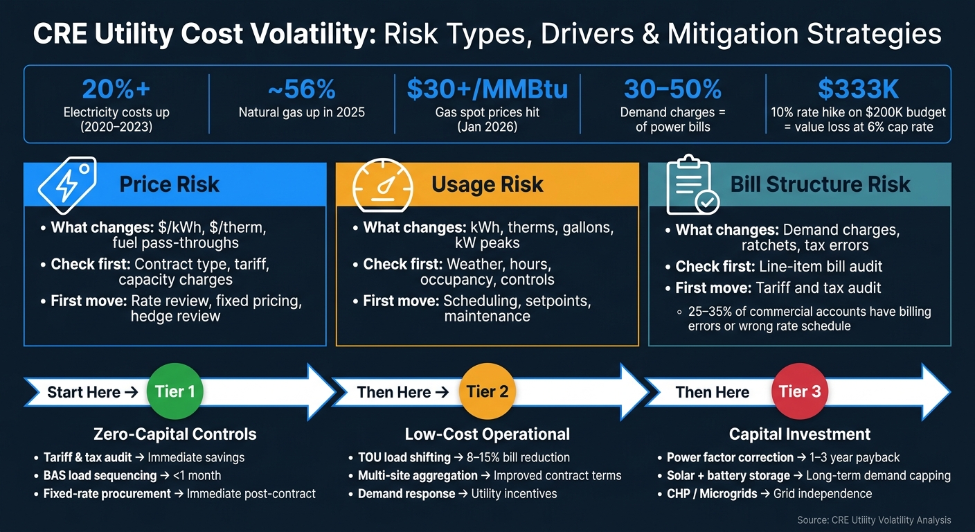
- Electricity costs climbed 20%+ from 2020 to 2023
- Natural gas prices were up about 56% in 2025
- A short weather event in January 2026 pushed gas spot prices above $30/MMBtu
- Demand charges can make up 30% to 50% of a power bill
- A simple 10% electricity increase can add $3,600 to $6,000 a year at a 15,000 sq. ft. retail site
- On a $200,000 utility budget, that same 10% increase can cut value by about $333,000 at a 6.0% cap rate
So the playbook is simple:
- Split price changes from usage changes
- Pull 24 to 36 months of bills
- Normalize for weather and occupancy
- Review interval data for peaks and ratchets
- Stress test utility spend in underwriting
- Start with low-cost fixes before capex or procurement moves
The main cost drivers are usually:
- Market moves in power and gas
- Capacity and grid charges
- Demand peaks and ratchet clauses
- Weather and occupancy swings
- Setpoint drift, weak scheduling, and delayed repairs
- Bad tariffs, billing errors, or the wrong rate class
If I wanted one clean takeaway, it would be this: don’t treat utility expense like a flat line item. It behaves more like a risk input that needs review at the meter, asset, and portfolio level.
A fast side-by-side view:
| Risk area | What changes | What I’d check first | First move |
|---|---|---|---|
| Price risk | $/kWh, $/therm, fuel pass-throughs | Contract type, tariff, capacity charges | Rate review, fixed pricing, hedge review |
| Usage risk | kWh, therms, gallons, kW peaks | Weather, hours, occupancy, controls | Scheduling, setpoints, maintenance |
| Bill structure risk | Demand charges, ratchets, tax errors | Line-item bill audit | Tariff and tax audit |
If utility costs are hard to forecast, budgets slip, reserves get used, and debt sizing can look better than it should. That’s why I’d build utility volatility into diligence, underwriting, and monthly variance review from day one.
CRE Utility Cost Volatility: Risk Types, Drivers & Mitigation Strategies
Where Utility Cost Volatility Comes From
Utility cost swings usually come from three places: market forces, building operations, and tariff design. You have to separate them first. If you don't, it's easy to treat a usage problem like a pricing problem, or blame the utility when the issue starts inside the building. Each source behaves in its own way, so the fix depends on where the volatility begins.
External Market and Regulatory Drivers
Natural gas still drives a big share of U.S. power generation. That means Henry Hub price swings often show up in commercial electric bills. In 2025, gas prices were up about 56% versus 2024 [2][4].
Capacity charges are putting more pressure on costs too. In the PJM Interconnection, capacity prices jumped tenfold for the 2025–2026 planning period, while MISO saw a twentyfold increase in that same window [3]. Those jumps reflect the cost of keeping the grid reliable as older fossil fuel plants retire and demand grows from data centers, AI infrastructure, and industrial electrification. ERCOT in Texas is also projecting nearly 10% demand growth in 2026 [2].
Utility rate cases, regulated grid investment, and regional congestion can push costs higher even when fuel prices aren't moving much [2][3]. In some markets, local transmission bottlenecks make prices behave very differently from national averages. Global LNG disruptions and tariffs on energy components add another layer of price uncertainty [2][3][4].
Property Operations, Occupancy, and Equipment Performance
Market prices set the ceiling. Operations decide what you actually spend.
For retail-facing CRE such as QSRs, retail, and theaters, HVAC and refrigeration are often the biggest site-level energy loads [2][4]. When sites have operating issues like setpoint drift or weak runtime schedules, they often use 20% to 30% more energy per square foot than the portfolio average [2]. You won't spot that gap in a simple rate comparison. It shows up only when consumption data is normalized and benchmarked.
Deferred maintenance makes things worse. Repairs get pushed out, efficiency slips, and costs jump. It usually doesn't show up as a slow climb. More often, it hits as sudden spikes that weren't in the forecast. After-hours energy use from idle loads, like equipment running in empty spaces, is another common source of hidden waste. That problem usually gets caught only when someone is watching interval data on a regular basis.
Variable operating hours can also create month-to-month swings that look like price volatility even when they're just usage changes. Tracking energy cost per occupied hour, instead of raw consumption alone, helps separate one from the other. Normalized benchmarking is what shows whether the issue is price, usage, or both.
Tariffs, Contracts, and On-Site Energy Structures
Procurement structure can soften volatility or make it worse. Fixed-rate contracts, usually 12 to 36 months, lock in price certainty. Indexed or market-rate pricing leaves assets exposed to spot market events like Winter Storm Fern [2][5]. Fixed terms cut uncertainty, but they can also leave you paying more if market rates drop.
Demand charges are one of the least understood cost drivers in commercial real estate. They often make up 30% to 50% of a commercial electric bill, and they're driven by a single 15-minute peak interval during the billing period [5]. One bad startup sequence can reset the month's demand charge. Ratchet clauses make that hit linger by tying minimum billing demand to a share - often 60% to 90% - of the highest peak from the prior 12 months [5]. One rough month can keep costs high for a full year.
Fuel adjustment clauses (FAC) let utilities pass fuel cost changes straight through to customers. So a bill can go up month over month even when consumption is flat [5].
The table below shows the main volatility drivers, what they affect, and where the most practical mitigation levers sit:
| Volatility Driver | Affects Price or Consumption? | Common Mitigation Lever |
|---|---|---|
| Natural Gas Prices | Price | Fixed-rate procurement / Hedging |
| Capacity Charges | Price (Structural) | Peak load shedding / Demand response |
| Demand Charges | Price (per kW) | Load sequencing / Battery storage |
| Ratchet Clauses | Price (Long-term) | Peak demand limiting / Tariff review |
| Extreme Weather | Consumption & Price | Weather normalization / Thermal storage |
| Time-of-Use (TOU) Rates | Price (Variable) | Load shifting to off-peak |
| Deferred Maintenance | Consumption | Predictive maintenance / Real-time monitoring |
| Setpoint Drift | Consumption | Remote setpoint locking / EMS controls |
| Grid Congestion | Price (Regional) | Load shifting / Distributed energy |
One common blind spot: an estimated 25% to 35% of commercial utility accounts have billing errors or sit on the wrong rate schedule entirely [5]. That's not a small miss. It's a steady source of overpayment that a basic tariff audit can often surface fast.
That driver map becomes the starting point for bill-level normalization and benchmark testing.
sbb-itb-df8a938
Due Diligence: How to Measure Utility Cost Exposure Before It Hurts NOI
Once you know the main cost drivers, the next move is simple: measure exposure at the meter level before it shows up in NOI. That means pulling meter-level data that shows what the property is actually using and what it's actually paying.
Utility Bill Collection, Normalization, and Anomaly Review
Start with 24–36 months of utility bills for every account, split by meter and utility type. You want to see trends in kWh, therms, gallons, and demand charges. But don't stop at the headline numbers. Look closely at line items like power factor penalties and fuel adjustment clause (FAC) charges. At the same time, check for billing errors, tariff mismatches, and missed exemptions.
Raw usage data, by itself, doesn't tell you much. Normalize the data with heating and cooling degree days (HDD/CDD) so weather swings don't muddy the picture. Then adjust for occupancy shifts and one-time events. For retail or QSR properties, energy cost per transaction ties utility spend to sales activity. For hospitality, cost per occupied room (POR) helps strip out distortion from occupancy swings. Once the numbers are normalized, the outliers tend to stand out. That's when you can flag sites with steady variance against peer benchmarks.
Also ask the utility for 15- or 30-minute interval load data [5]. This is where things get more interesting. It can show peak demand events, ratchet exposure, and time-of-use (TOU) savings room. A single high-demand event during a renovation can lock in higher demand charges for the next 12 months under a ratchet clause, and you may not spot that in a standard monthly bill summary. That kind of view helps you see whether the property needs an operating fix, a tariff change, or both.
The point is to separate market-driven rate risk from building-driven usage risk before underwriting.
Benchmarking and Stress Testing for Underwriting and Lender Review
After normalization, compare each asset to its own past performance and to other assets in the portfolio. Benchmarking helps sort out building-level problems from short-term market noise. Energy per square foot is the usual cross-site metric. For properties with uneven hours, cost per occupied hour is often a better fit.
From there, model three utility cost cases for underwriting:
| Scenario | Assumption | NOI Impact to Model |
|---|---|---|
| Base Case | 12-month trailing average + 10–15% buffer | Reflects expected volatility range [2] |
| Moderate Stress | Sustained utility rate increase | Tests margin compression under a tougher pricing environment |
| Severe Stress | Winter Storm Fern (Jan. 2026) | Stress-tests DSCR and debt sizing under extreme conditions [2] |
These cases turn utility volatility into something you can model in NOI and DSCR. Use a severe market shock to test DSCR and debt sizing under extreme conditions. Then run that stress case through NOI and DSCR so lenders can see the risk has been modeled, not brushed aside.
Using Structured Analytics and Monitoring Tools
Use analytics tools to automate bill ingestion, normalization, and variance tracking across the portfolio.
When you combine bill-level data, normalized benchmarking, and scenario modeling, you get a clear view of utility risk that buyers, lenders, and asset managers can defend under scrutiny. And once exposure is quantified, the next step is to reduce volatility through controls, capital projects, and procurement.
How to Reduce Utility Cost Volatility: Controls, Capital, and Procurement
Once you’ve measured exposure, the next move is simple: start with no-cost or low-cost controls, then look at capital projects, and only then move to procurement. The goal is to go after the biggest cost drivers you can actually control.
Low-Cost Controls and Tenant-Facing Measures
Begin with zero-capital controls.
A tariff and tax audit should come first because it can lead to savings right away.
If your utility bill includes demand charges or ratchets, stagger equipment starts over 10 to 15 minutes to lower the monthly peak. That’s one of the most direct ways to limit swings in consumption costs. In retail and QSR properties, the biggest pressure points are often HVAC runtime schedules and setpoint drift. In large office and industrial buildings, it usually makes more sense to watch power factor correction and ratchet clause exposure closely [5].
Under TOU pricing, shifting 15% to 20% of load to off-peak hours can reduce total bills by 8% to 15% [5].
If those steps don’t do enough to steady costs, the next step is capital work aimed at peak demand or exposure to price swings.
Capital Projects and On-Site Energy Investments
Capital projects work best when they go straight at demand charges or limit exposure to peak pricing events.
For buildings with heavy HVAC use or large motor loads, power factor correction can cut utility penalties. This usually means installing capacitor banks when power factor falls below the 0.85 to 0.95 range. Typical payback is one to three years [5].
Battery energy storage is one of the clearest tools for peak shaving because it can cap billed demand when demand charges are high [5]. Solar by itself doesn’t always fix volatility, since output may not line up with peak demand periods. But solar paired with storage can do a better job of capping demand and lowering net consumption [5].
For properties in markets dealing with steep capacity price jumps, distributed energy setups like combined heat and power (CHP) or microgrids can help buffer the asset from capacity market spikes and grid reliability problems [3].
When operating changes can’t absorb enough of the volatility, procurement becomes the next lever.
Tariff Selection, Procurement, and Hedging
On the procurement side, keep an eye on natural gas futures and look at fixed contracts during late summer or mild-weather periods, when storage is high and pricing pressure is lower [2]. Fixed-rate contracts usually run 12 to 36 months and give price certainty as soon as the contract is in place [5][2].
Financial hedging tools can offer similar protection, though premiums may climb when volatility gets worse [3].
For larger portfolios, multi-site aggregation gives you more negotiating power than buying for one asset at a time. Rolling load from several properties into one procurement structure can improve contract terms and make site-level outliers easier to spot [2].
Demand response can add one more layer of protection. Utilities pay incentives when customers reduce usage during periods of peak grid stress [3].
| Strategy | Impact on Volatility | Capital Intensity | Implementation Complexity | Time to Benefit |
|---|---|---|---|---|
| Tariff/Tax Audit | High (cost reduction) | Zero | Low | Immediate |
| BAS Load Sequencing | High (demand) | Low | Low | < 1 month |
| TOU Load Shifting | Moderate (unit cost) | Low | Medium | 1–3 months |
| Fixed-Rate Procurement | High (unit cost) | Zero | Medium | Immediate (post-contract) |
| Multi-site Aggregation | Moderate | Low | Medium | Short-term |
| Demand Response | Moderate | Low to medium | Medium | Short-term |
| Power Factor Correction | Low (penalty removal) | Medium | Medium | 1–3 year payback |
| On-site Storage / Solar + Storage | High (demand + consumption) | High | High | Long-term |
Use the table to line up each tactic with your budget, timeline, and the kind of volatility you’re trying to reduce. Start with zero-capital controls, then move into capital projects only where cost swings continue.
Embedding Utility Volatility into Underwriting, Asset Management, and Portfolio Decisions
Use the due-diligence outputs to set underwriting assumptions and portfolio thresholds.
Underwriting Assumptions, Sensitivities, and Debt Sizing
A flat 2% to 3% expense growth rate across all utilities doesn't hold up. Electricity, gas, and water move differently, so they shouldn't share one assumption. Take what you found in due diligence and turn it into utility-specific escalation rates, plus downside cases, in the pro forma.
The numbers make that pretty clear. Natural gas expenditures for some commercial assets grew at a CAGR of 6.7% between 2019 and 2023 [1], while commercial electricity rates increased by more than 20% per kWh from 2020 to 2023 [1]. If you model electricity, gas, and water separately, your NOI forecast is far less likely to drift off course.
For assets with strong seasonal swings, like self-storage or hotels, a single annual utility figure can hide too much. Model utilities across 12 monthly columns instead. Peak months and slow months can skew projections in a big way [7].
This matters for debt sizing too. If utility costs are understated, NOI and DSCR look better than they are, which can push lenders and buyers toward aggressive leverage [6]. Even a modest change can bite: a 10% electricity cost increase on a $200,000 annual utility budget reduces implied asset value by more than $330,000 at a 6% cap rate [8]. That sensitivity should be in front of lenders and investment committees from day one.
Portfolio Governance and Variance Management
At the portfolio level, use the same price-versus-consumption split to decide where attention and capital should go first.
Start by ranking assets by energy intensity, measured as kWh per square foot. Focus first on properties sitting well above the portfolio average [2]. Then review variance each quarter and split it into two buckets: price risk and consumption risk. That tells you where the problem lives. Is the issue procurement? Or is the building simply using more energy than it should?
Keep the KPI set small and consistent across acquisitions, asset management, property management, and finance. The goal is simple: everyone should be looking at the same scorecard.
- Energy cost per square foot for cross-site benchmarking
- Cost per occupied hour to tie spend to actual building use
- Weather-normalized kWh to remove seasonal distortion
- Peak demand charges to spot load-shifting opportunities [2]
Using the same metrics across teams cuts down on confusion and makes handoffs cleaner.
| Lifecycle Stage | Analytical Tool / Process | Owner | Primary Output |
|---|---|---|---|
| Acquisition / Underwriting | Utility-specific escalation models, sensitivity tables | Acquisitions / Analyst | Stressed NOI, DSCR, debt sizing |
| Due Diligence | Bill normalization, weather-adjusted benchmarking | Asset Management / Analyst | Exposure score, anomaly flags |
| Asset Management | Monthly KPI tracking, variance reporting | Asset / Property Management | Budget variance explanation |
| Portfolio Review | Energy intensity ranking, scenario modeling | Finance / Portfolio Management | Capital prioritization, hold-sell input |
| Disposition / Refinance | Utility cost trend analysis, lender reporting | Finance / Analyst | Adjusted valuation, lender reporting |
Conclusion: Core Steps CRE Teams Should Standardize
The CRE teams that handle utility cost volatility well tend to do a few things the same way every time. They split price risk from consumption risk. They collect and normalize utility data before it turns into a budget issue. And they stress test utility expense in underwriting instead of waiting until after closing.
They also pick mitigation tactics based on the asset in front of them, not by habit. That may mean operational controls, capital projects, procurement moves, or some mix of the three, depending on the property's load profile and capital plan.
Just as important, they keep watching variance at both the property and portfolio level so small misses don't snowball into material NOI erosion.
When utility volatility becomes part of the standard financial process, teams are in a stronger spot to protect margins and make smarter capital calls across the full asset lifecycle. That's getting more important as demand growth, weather extremes, regional grid constraints, and global fuel market uncertainty make utility costs harder to forecast than they were even three or four years ago.
FAQs
How do I tell price risk from usage risk?
Price risk comes from market-driven swings in utility rates. So it’s worth tracking rate changes over time and building room in your budget for volatility.
Usage risk comes from changes in consumption. To keep an eye on it, watch metrics like energy use per square foot or per transaction. That helps you spot shifts in efficiency or demand that aren’t tied to price changes alone.
Which utility data should I collect before underwriting?
Collect utility data from:
- landlord-controlled spaces
- whole-building systems through automated access or the utility company
- tenant spaces through data-sharing agreements or direct access
This gives you a more complete and accurate view of energy performance.
What are the fastest, low-cost ways to cut utility volatility?
The fastest, low-cost ways to cut utility volatility usually come down to planning and day-to-day operations, not big capital projects.
Two moves matter right away. First, use blended rate forecasting with a 10–15% buffer above the 12-month trailing average. That gives you a more realistic cushion instead of betting on flat pricing. Second, apply weather normalization so you can tell the difference between swings caused by weather and actual changes in efficiency. Without that step, it’s easy to misread the numbers.
A few other steps can help too:
- Multi-site aggregation planning can improve procurement leverage across locations.
- Procurement timing awareness matters, especially when it makes sense to lock in rates as natural gas futures trend lower, often in late summer.
These are not flashy changes. But they can take a lot of the guesswork out of utility costs and make budgeting less of a roller coaster.